Gait as a Password
11 June 2026Gait as a Password: Building a Biometric Authentication System with Deep Learning
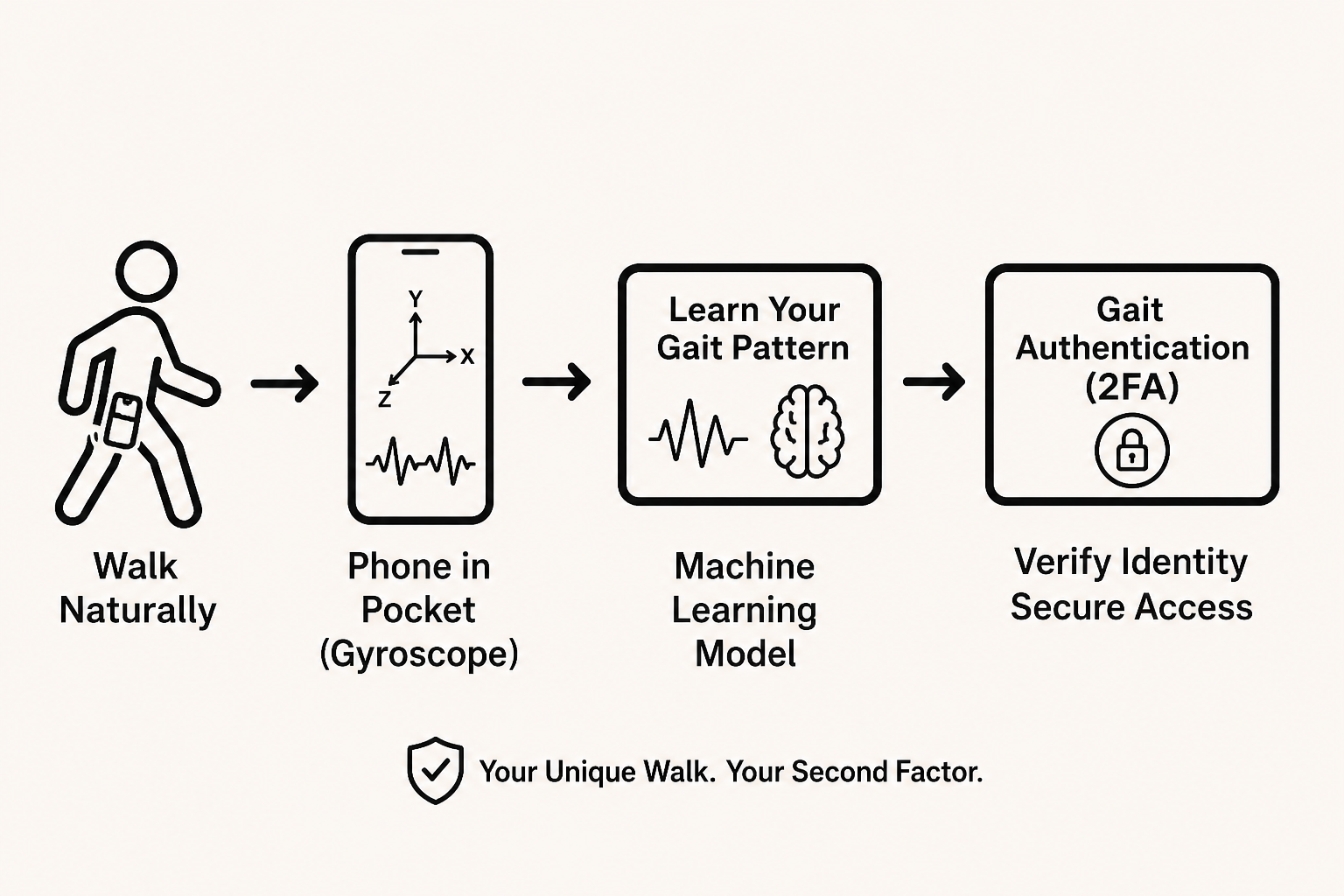
Your smartphone already knows how you walk. Every step generates a unique pattern of acceleration and rotation — a gait signature as distinctive as your fingerprint. The accelerometer and gyroscope inside your phone track these micro-movements at 50 Hz, producing a 6-dimensional time series that encodes your personal walking style.
This post walks through how we built an open-set gait authentication system using deep metric learning. The system learns an embedding space where same-person gaits cluster together, and different-person gaits stay apart — all without ever seeing the person during training. You can try the live demo at gait-authentication.sigurdurhaukur.com.
Why Bother? MFA Is Broken
Most multi-factor authentication boils down to three categories: something you have (a key, a phone, a bracelet — can be lost or stolen), something you know (a password or PIN — phishable and interceptable), and something you are (face, fingerprint — usually requires a deliberate action like pressing a sensor or looking at a camera).
Gait is a fourth option that sidesteps the weaknesses of the other three: it’s passive (no user action needed — you’re already walking with your phone), impossible to phish (there’s no secret to leak), and unforgettable (you can’t lose your own walk). It runs on hardware nearly everyone already carries.
The Problem
Gait recognition is harder than it sounds. Walking patterns vary with speed, terrain, footwear, fatigue, and even mood. The sensor data is noisy — a phone in a pocket jostles differently than one held in hand. On top of that, the system must operate in an “open-set” setting: it needs to authenticate users it has never encountered during training.
The dataset is the Gait-Datasets-TIFS20 Dataset #1, containing 6-channel IMU signals (3-axis acceleration + 3-axis gyroscope) from 175 participants walking with a smartphone in their pocket. Each participant has a single recording of roughly 20,000 timesteps at 50 Hz — about 6–7 minutes of walking.

The Solution: Metric Learning in a Nutshell
Instead of training a classifier that recognizes specific people (which fails when new users appear), we learn an embedding function — a neural network that maps a gait window to a point on the unit hypersphere in 64-dimensional space. The key property: windows from the same person map to nearby points, while windows from different people map far apart.
At authentication time, the user walks for 30–60 seconds. Their sensor data is split into windows, each window is encoded into an embedding, and the average embedding is compared to the stored enrollment centroid. If the L2 distance falls below a threshold, they’re authenticated.
This is a classic open-set protocol: during evaluation, half the held-out participants are “enrolled” (their centroids are computed), and the other half act as impostors. We sweep the distance threshold to find the Equal Error Rate (EER) — the point where False Acceptance Rate equals False Rejection Rate.
Architecture
We implemented two neural architectures plus a non-learning baseline:
1. Transformer Encoder
class GaitTransformer(nn.Module):
    def __init__(self, input_size=6, d_model=64, nhead=4,
                 num_layers=2, dim_feedforward=128,
                 embedding_size=64, dropout=0.01):
        super().__init__()
        self.input_projection = nn.Linear(input_size, d_model)

        encoder_layer = nn.TransformerEncoderLayer(
            d_model=d_model, nhead=nhead,
            dim_feedforward=dim_feedforward,
            dropout=dropout, batch_first=True,
            activation="gelu",
        )
        self.encoder = nn.TransformerEncoder(
            encoder_layer, num_layers=num_layers
        )
        self.dropout = nn.Dropout(dropout)
        self.embedding_head = nn.Linear(d_model, embedding_size)

    def forward(self, x):
        x = self.input_projection(x)
        x = self.encoder(x)
        x = x.mean(dim=1)          # Pool over time
        x = self.dropout(x)
        embedding = self.embedding_head(x)
        return F.normalize(embedding, p=2, dim=1)
The input projection maps 6 raw sensor channels into a 64-dimensional space. A 2-layer Transformer encoder with 4-head self-attention learns which timesteps are most discriminative. Mean pooling across the sequence collapses time, and the final linear layer projects to the 64-D embedding, L2-normalized onto the unit sphere.
Honest confession: we forgot to add positional encodings. Self-attention is permutation-invariant by design, so our Transformer technically treats each gait window as a bag of timesteps. The model still converged and achieved the best results, which either means the temporal structure is encoded implicitly in the signal amplitudes, or — more likely — that we left a clear improvement on the table.
2. Bidirectional LSTM
class LSTM(nn.Module):
    def __init__(self, input_size=6, hidden_size=128,
                 num_layers=2, embedding_size=64,
                 dropout=0.01):
        super().__init__()
        self.lstm = nn.LSTM(input_size, hidden_size,
                            num_layers, batch_first=True,
                            dropout=dropout if num_layers > 1 else 0)
        self.dropout = nn.Dropout(dropout)
        self.fc = nn.Linear(hidden_size, embedding_size)

    def forward(self, x):
        lstm_out, _ = self.lstm(x)
        last_output = lstm_out[:, -1, :]   # Last timestep
        last_output = self.dropout(last_output)
        embedding = self.fc(last_output)
        return F.normalize(embedding, p=2, dim=1)
A 2-layer LSTM with 128 hidden units reads the sequence and uses only the final timestep’s hidden state for the embedding.
We compared four approaches to triangulate how much of the performance comes from learned representations versus the evaluation protocol itself:
| Method | Rationale |
|---|---|
| Random Baseline | Just randomly guess if it’s an enrolled user (≈50% EER) |
| FFT + Centroid | Simple baseline using hand-engineered frequency features |
| LSTM | Simple sequence model, initially our main model before testing transformers |
| Transformer | Captures fine-grained temporal patterns via self-attention |
3. FFT Centroids (Baseline)
A non-neural baseline: each 128-timestep window is transformed via FFT, the first 250 magnitude coefficients per channel are concatenated (1500 total), and features are selected by 95% cumulative energy. A StandardScaler normalizes the features, and enrollment is simply the per-user mean. This requires no GPU training and serves as the fast inference option in the API.
Training Pipeline
Data Processing
Each participant’s raw recording (~20,000 timesteps × 6 channels) is split into non-overlapping windows of 128 timesteps (~2.56 seconds at 50 Hz). This produces roughly 150 windows per participant.
Participants are split deterministically (seed=67) into 70/15/15 train/val/test, ensuring no participant appears in more than one split. A StandardScaler is fitted per fold on training windows only — a critical detail to prevent data leakage.

We experimented with three preprocessing filters — a 4th-order Butterworth low-pass at 5 Hz, a Kalman filter, and an FFT-based low-pass — but found they offered no consistent improvement over raw signals for the neural models. The networks learned to ignore high-frequency noise on their own.
Loss Functions
We experimented with two loss functions:
Online Triplet Loss: For each batch, we mine semi-hard triplets — anchor-positive pairs with a negative that is farther than the positive but within the margin. If no semi-hard negative exists, we fall back to the hardest negative.
def mine_semihard_triplets(embeddings, labels, margin):
    dist_mat = torch.cdist(embeddings, embeddings, p=2)
    for label in unique_labels:
        pos_mask = labels == label
        # For each anchor-positive pair in this class...
        for a_idx, p_idx in pos_pairs:
            ap_dist = dist_mat[a_idx, p_idx]
            semi_hard = (neg_dists > ap_dist) & (neg_dists < ap_dist + margin)
            # Select semi-hard negative, or hardest if none found
CosFace Loss: A normalized linear layer with additive angular margin penalty. The classifier weights are L2-normalized class prototypes, and a margin is subtracted from the correct class logits before softmax. This avoids the expensive triplet mining step and provides more stable training.
K-Fold Cross-Validation
The development set (train + val) undergoes 5-fold participant-wise cross-validation. Each fold: 1. Fits scaler on fold’s training windows 2. Trains the model with early stopping (patience=5 epochs) 3. Computes validation EER after each epoch via open-set evaluation 4. Restores the best model checkpoint
After CV, the model is retrained on the full development set and evaluated on the held-out test set.
Evaluation Protocol
The open-set evaluation splits held-out participants into “known” (enrolled) and “unknown” (impostors). For each of 10 resamples:
- Randomly split each known participant’s windows: half for enrollment centroid, half as probes
- Unknown participants: all windows are probes, scored against their nearest centroid
- Sweep 100 thresholds to find EER
This simulates the real-world scenario: users enroll once, then attempt authentication later, while impostors with no enrollment try to get in.
Results
The Transformer model with CosFace loss significantly outperformed both the LSTM and the FFT + Centroid baseline across all metrics.
| Authentication Method | Validation EER ± SEM | Hold-out Test EER | Test FAR | Test FRR |
|---|---|---|---|---|
| Transformer | 5.60% ± 0.73% | 4.02% [0.56%, 7.27%] | 3.96% | 4.07% |
| LSTM | 13.40% ± 1.17% | 11.16% [3.77%, 18.73%] | 11.11% | 11.21% |
| FFT + Centroid Baseline | 32.98% ± 3.92% | 38.94% [23.37%, 53.33%] | 31.01% | 46.88% |
| Random Guessing | — | 53.48% | 53.63% | 53.34% |
Note: Lower EER indicates superior performance. EER balances False Acceptance Rate (FAR) and False Rejection Rate (FRR). Participant-level evaluation ensures results generalize to new users. Bracketed ranges show 95% confidence intervals.
The Transformer’s 4.02% test EER means that at the optimal threshold, roughly 4 out of 100 impostor attempts are falsely accepted and 4 out of 100 legitimate attempts are falsely rejected — a 3× improvement over the LSTM and nearly 10× over the FFT baseline. Both neural models substantially outperform random guessing (53.48% EER), confirming that gait carries genuine biometric signal.
The Transformer outperforms the LSTM by a wide margin — 4.02% vs 11.16% test EER. We attribute this to self-attention’s ability to model long-range dependencies in the gait cycle. The LSTM compresses the entire 128-timestep window into a single hidden state, while the Transformer maintains per-timestep representations and pools them only at the end.
The FFT + Centroid baseline (38.94% EER) shows that simple frequency-domain features capture some gait information but are far from sufficient for reliable authentication. The high FRR (46.88%) means nearly half of legitimate users would be rejected at the threshold that balances the two error types.


API and Deployment
We packaged the system as a FastAPI application with three model options:
| Endpoint | What it does |
|---|---|
POST /models/{type}/encode-recording |
Convert 6-channel sensor data → 64-D embedding |
POST /models/{type}/authenticate |
Compare embedding to reference → match/no-match |
POST /embeddings/plot |
Generate t-SNE visualization of auth history |
Models are loaded from Hugging Face Hub
(slugroom/gait-classification-models) with local file
fallback. The API preloads all available models on startup via the
lifespan context.
The web frontend is a mobile-first SPA using HTMX and the DeviceMotionEvent API. Users select a model, walk for 60 seconds to enroll, then authenticate with a 30-second walk. The embedding is stored in localStorage, and authentication results appear as an overlay with distance and confidence scores. Real-time gyroscope visualization renders a tilt dot on a Canvas, and the Web Audio API provides countdown beeps and haptic feedback.
Interesting Findings
1. The Transformer dominates the LSTM
The Transformer (4.02% test EER) outperforms the LSTM (11.16%) by nearly 3×. Both use the same embedding size, the same loss function, and the same data pipeline. The difference comes down to representation: the LSTM compresses the entire 128-timestep window into a single hidden vector, while the Transformer maintains per-timestep representations throughout and pools via a learned mean. Self-attention can selectively focus on the most discriminative phases of the gait cycle — the heel strike, the toe-off, the mid-swing — rather than drowning them in the average.
2. The FFT baseline is weak
The FFT + centroid method (38.94% test EER) barely beats random guessing (53.48%). This surprised us — frequency-domain features often work well for motion recognition. But for fine-grained person identification, the crude energy-based feature selection discards too much information. The neural models are not just refining the same features; they are learning fundamentally different representations from the raw time domain.
3. CosFace outperformed triplet loss in practice
While triplet loss is theoretically elegant, CosFace provided more stable convergence and was less sensitive to hyperparameters. The online triplet mining produced no triplets in roughly 5% of batches (when a batch contained too few samples per class), stalling learning. CosFace always produces a gradient, since every batch contributes to the classification loss.

The triplet margin sweep reveals that performance is sensitive to this hyperparameter — too small and negatives are too easy, too large and training becomes unstable.
4. The embedding space is surprisingly low-dimensional
The finetuning grid search showed that 16-D or 32-D embeddings produce nearly identical EER to 64-D, suggesting the true intrinsic dimensionality of gait patterns is quite low. A 16-D embedding vector is only 64 bytes — compact enough to store hundreds of user profiles in a browser’s localStorage.
5. Some participants are just hard to distinguish
The hold-out test EER of 4.02% masks considerable variation across individuals (95% CI: 0.56%–7.27%). Some participants have highly distinctive walks; others walk in a way that’s close to the population average. This is well-documented in the biometrics literature — it’s called the “sheep, goats, and lambs” problem (users who are easy to recognize, hard to recognize, and easy to spoof).
6. Real-world sensor data is messy
The original dataset was collected in controlled conditions (same pocket, same walking speed, same surface). In our live demo, we observed that people using the system in the real world get higher EER because they vary their walking speed, hold their phone differently, or walk on different surfaces. The gap between lab accuracy and real-world accuracy is substantial — a challenge shared by every biometric modality.
7. Explainability: the F-ratio spectrum
We computed the F-ratio (between-class variance / within-class variance) for each frequency bin to understand what the model actually learns:

The spectrum reveals that the most discriminative information concentrates in the 0–10 Hz range — roughly the natural frequency band of human walking. Above 10 Hz the signal is mostly noise, confirming that the Butterworth filter’s 5 Hz cutoff was reasonable and that the Transformer is effectively learning a data-driven frequency selection.
A PCA projection of the class centroids (64-D → 2-D) further confirms that the learned embedding space separates participants well:

8. An untrained Transformer already beats the FFT baseline
As a sanity check, we ran the open-set evaluation on a Transformer with random, untrained weights. It scored 21.62% ± 11.17% EER — clearly not usable, but already much better than the 38.94% FFT + Centroid baseline and miles better than the 53.48% random-guessing reference. A random projection into a 64-D space apparently preserves enough structure for centroid-based matching to do something. Getting a workable embedding space (around 10-20% EER) came fairly easily during training; the real effort went into pushing from there down below 5% via CosFace tuning and architecture choices.
Risks and Limitations
Honesty about what could go wrong matters as much as the headline numbers:
- Distribution shift in deployment. The dataset was collected with a phone in a fixed pocket position and orientation. Real users hold phones in hands, bags, or different pockets, which our live demo confirmed degrades accuracy.
- Gait is not static. Footwear, injury, fatigue, and carrying bags or children all change how a person walks — and our model has no mechanism to adapt to this over time.
- False acceptances are security-critical. In a real deployment the threshold should be tuned to favor lower FAR (fewer impostors let in) even at the cost of higher FRR (more legitimate users asked to re-authenticate), which is the opposite of how we tuned for EER.
- Dataset size is limited for biometric deployment. 175 participants is enough to demonstrate feasibility but small relative to production-scale biometric systems.
- Regulatory reality. Gait is biometric data. A real product would need privacy, consent, security, and regulatory review (e.g., GDPR considerations for biometric identifiers) — work that is out of scope for a course project but would be a hard requirement before any real-world use.
Lessons Learned
Building a gait authentication system taught us that biometrics is as much about the evaluation protocol as the model architecture. The open-set, centroid-based evaluation forced us to think carefully about enrollment quality, distance thresholds, and the tradeoff between security and convenience.
The full source code is available on GitHub. If you want to train your own model:
# Quick test with 500 samples
python -m gait_classification.train max_samples=500 model_type=transformer

# Full training with CosFace loss
python -m gait_classification.train model_type=transformer num_epochs=20
Or deploy the API:
uvicorn gait_classification.api:app --reloadThe live demo is at gait-authentication.sigurdurhaukur.com — grab your phone and see if your walk is as unique as you think.